
The Psychological Tightrope of Position Sizing
I remember the first time I realized that my entry signal was almost irrelevant. I had spent months perfecting a crossover strategy that promised an 65% win rate. On paper, I was going to be a millionaire by Christmas. In reality, three weeks into live trading, my account was down 40%. The problem wasn’t the strategy; it was my ego. I was betting 20% of my account on every trade because I was ‘sure’ it would work.
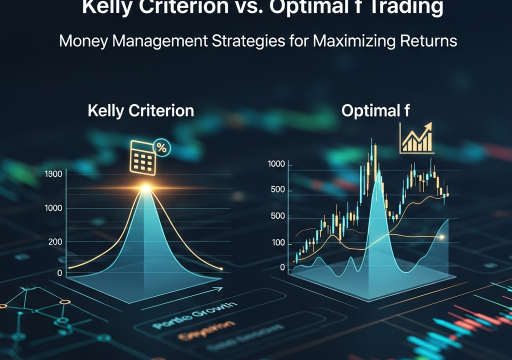
This is where the debate of Kelly Criterion vs Optimal f trading begins. Most traders focus on *what* to buy, but successful traders focus on *how much* to buy. If you bet too little, you waste the potential of your edge. If you bet too much, you’ll eventually hit a string of losses that wipes you out, even if your strategy is technically profitable. Finding that ‘Goldilocks’ zone—the perfect fraction of your capital to risk—is what separates the legends from the gamblers.
As we navigate the markets in 2026, where algorithmic volatility can shift in milliseconds, understanding these mathematical frameworks is more vital than ever. We aren’t just fighting human sentiment anymore; we are fighting optimized machines. To survive, your risk management needs to be just as optimized.
The Birth of the Kelly Criterion
The story of the Kelly Criterion doesn’t start on Wall Street. It starts at Bell Labs in 1956. John Kelly was a scientist looking at long-distance telephone signal noise. He realized the same math used to transmit information across noisy channels could be applied to gambling. If you have an edge (even a tiny one) and you know the odds, there is a specific percentage of your bankroll that will maximize your long-term growth rate.
The beauty of Kelly is its simplicity. In a binary world—like a coin flip or a simple sportsbook bet—the formula tells you exactly what to do. You take your win probability and your payout ratio, plug them in, and out pops a number. If that number is 0.05, you bet 5% of your account. It’s elegant, it’s mathematically sound, and it’s the foundation for almost every serious quantitative strategy used today.
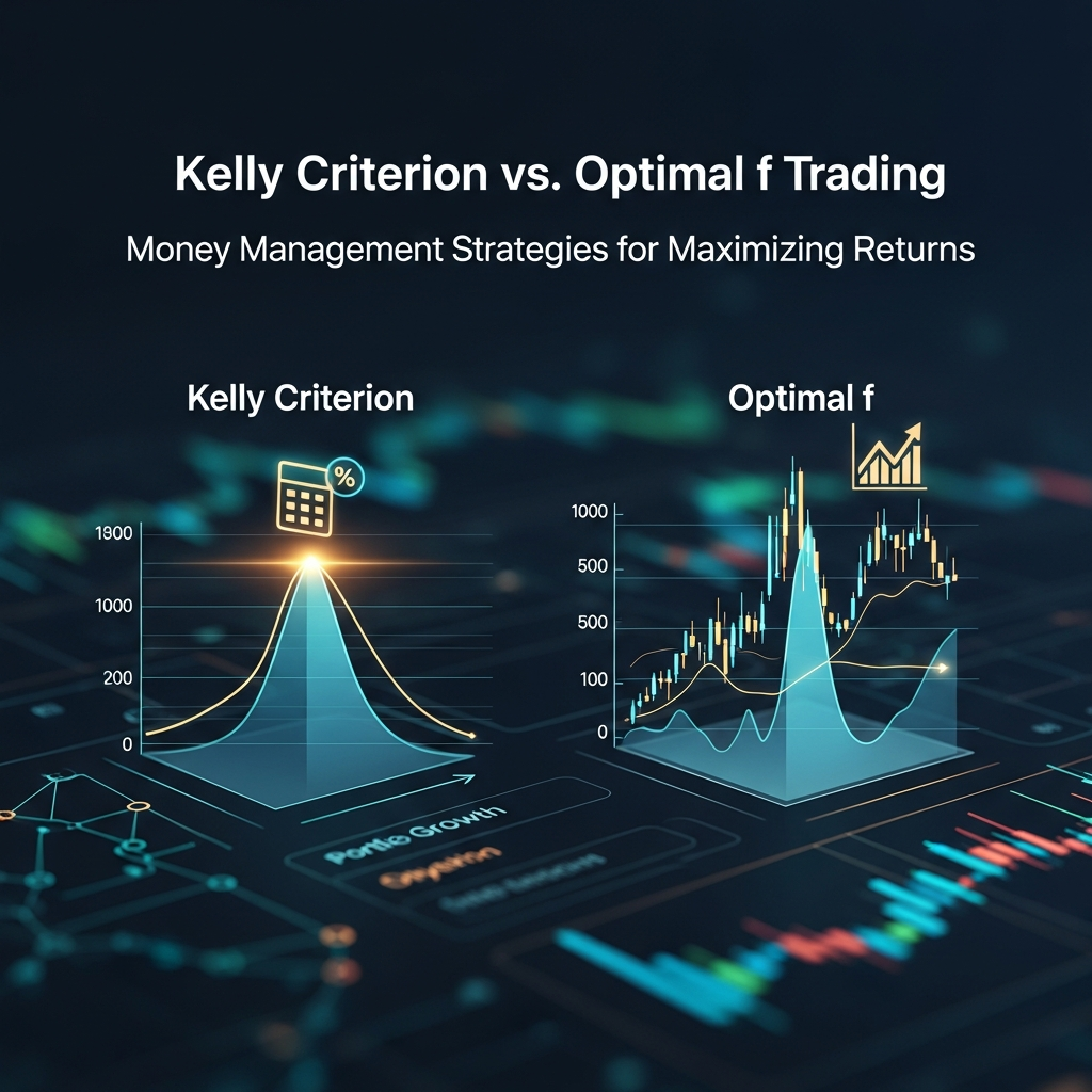
However, the Kelly Criterion makes a massive assumption: that the outcomes are binary (win or lose) and the odds are fixed. In the messy world of the S&P 500 or Bitcoin, trades don’t just ‘win’ or ‘lose.’ You have small wins, massive outliers, tiny losses, and the occasional ‘black swan’ event that ruins your day. This is the primary friction point when comparing Kelly Criterion vs Optimal f trading.
The Formula at a Glance
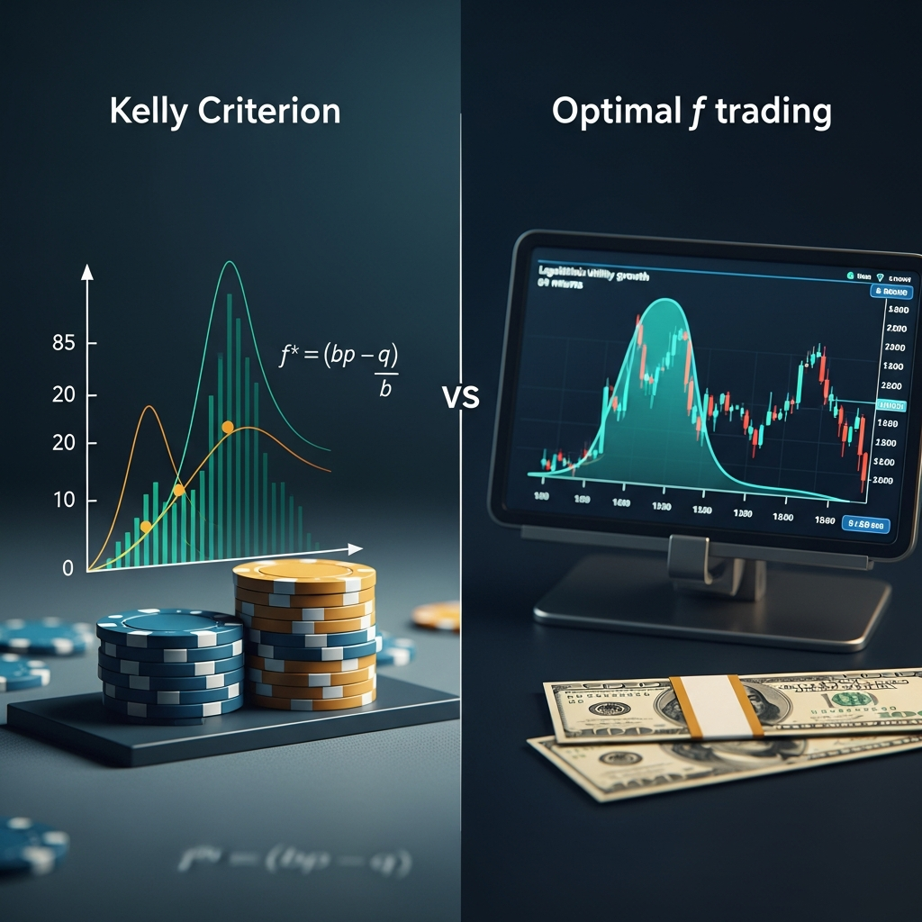
For those who love the numbers, the basic Kelly formula looks like this: f* = (bp – q) / b. Here, f* is the fraction of the bankroll to bet, p is the probability of winning, q is the probability of losing (1-p), and b is the decimal odds. It looks great on a whiteboard. But when you’re staring at a volatile chart in the middle of a Tuesday session, its rigid structure can feel a bit disconnected from reality.
Ralph Vince and the Evolution into Optimal f
Enter Ralph Vince. In the late 1980s and early 90s, Vince took Kelly’s work and dragged it into the real world of professional trading. He recognized that trading isn’t a series of coin flips. A single trade could lose $100, $500, or $5,000 depending on where your stop loss is or if the market gaps against you. He introduced the concept of ‘Optimal f.’
The ‘f’ stands for fraction. Specifically, the fixed fraction of your capital that you should risk on a given unit of your trading system. Unlike Kelly, which often relies on the *average* win/loss, Optimal f is derived from your actual historical trade distribution. It looks at the sequence of your past trades and calculates the exact fraction that would have yielded the highest ‘Terminal Wealth Relative’ (TWR).
When you look at Kelly Criterion vs Optimal f trading, Optimal f is essentially Kelly’s more sophisticated, street-smart cousin. It doesn’t care about theoretical probabilities; it cares about what actually happened in your trade log. It accounts for the varying sizes of your wins and losses, making it much more applicable to a diversified portfolio or a complex trend-following system.
Breaking Down the Mechanics: Kelly Criterion vs Optimal f trading
To really understand the difference, we have to look at how they handle ‘lumpiness’ in data. Trading is inherently lumpy. You might have ten small wins and one giant loss, or twenty small losses and one massive home run.
- The Rigidity of Kelly: Kelly works best when the payout is symmetric or easily defined. Because it often uses averages (Average Win / Average Loss), it can sometimes underestimate the risk of a strategy that has ‘fat tails’—those rare but devastating losses that exceed your historical average.
- The Empirical Nature of Optimal f: Optimal f is purely empirical. It doesn’t assume a normal distribution. If your history shows a catastrophic outlier, Optimal f will see that and drastically reduce your suggested risk fraction to ensure you survive another one.
In the debate of Kelly Criterion vs Optimal f trading, the winner often depends on your data quality. If you have thousands of trades and a stable edge, Optimal f is incredibly powerful. If you are starting out or have a limited data set, the Kelly Criterion offers a safer, more theoretical starting point.
The Hidden Trap: The ‘Blow-Up’ Risk
Here is the scary truth about both methods: they are aggressive. Mathematically, ‘Optimal’ means the point just before you start losing money due to volatility drag. If you bet exactly at the Optimal f or full Kelly level, you are standing on the edge of a cliff. A slight shift in market regime—say, a sudden spike in correlation across your assets—can move your ‘optimal’ point lower. If you are still betting at the old level, you are now over-leveraged.
I’ve talked to traders who tried to run ‘Full Kelly.’ Their equity curves look like a rocket ship until they don’t. They usually end up hitting a 70% or 80% drawdown. Technically, they aren’t ‘ruined’ (as in, their account isn’t zero), but psychologically, they are done. Most humans cannot handle a 50% drop in their life savings, regardless of what the math says about the ‘long-term recovery.’
This is why the 2026 standard for professional desks isn’t full Kelly or full Optimal f. Instead, we use ‘Fractional Kelly’ or ‘Fractional f.’ Usually, this means taking the optimal number and dividing it by four (Quarter Kelly) or two (Half Kelly). This drastically reduces volatility and drawdowns while still capturing the lion’s share of the growth potential. It’s the pragmatic middle ground in the Kelly Criterion vs Optimal f trading saga.
Volatility Drag: The Silent Killer
Why do we care so much about these fractions? Because of volatility drag. If you lose 50%, you need a 100% gain just to get back to even. The more volatile your returns, the harder it is to grow your capital. Both Kelly and Optimal f are designed to find the point where growth is maximized relative to this drag. But remember, the ‘optimal’ point is the peak of a curve. If you go just a little bit past it, your growth rate doesn’t just slow down—it plummets.
Practical Implementation in 2026
How do you actually use this today? We aren’t calculating these by hand on napkins anymore. Most modern trading platforms and custom Python scripts can run Monte Carlo simulations to find your Optimal f in seconds. Here is a simplified workflow for choosing between Kelly Criterion vs Optimal f trading in your own setup:
- Step 1: Audit your Trade History. If you don’t have at least 50-100 trades, stick to a very conservative fixed-percentage risk (like 1%). You don’t have enough data for these formulas to be reliable.
- Step 2: Calculate your ‘f’. Use your largest loss as the divisor for Optimal f. This ensures that a repeat of your worst-case scenario won’t wipe you out.
- Step 3: Apply a Safety Buffer. Whatever number the Kelly Criterion vs Optimal f trading comparison gives you, cut it in half. If Kelly says risk 4%, risk 2%. You’ll sleep better, and your equity curve will be much smoother.
- Step 4: Monitor for Regime Change. Markets change. A strategy that worked in 2026 might have a different ‘optimal’ level in 2026. Re-run your calculations monthly.
The Final Verdict on Kelly vs Optimal f
If you are looking for a definitive winner, you might be disappointed. The truth is that they are two sides of the same coin. Kelly is the map, and Optimal f is the actual terrain. Kelly gives you the theory of how compounding works; Optimal f gives you the tool to apply that compounding to the messy, non-linear reality of price charts.
In my experience, the most robust traders use a hybrid approach. They use the Kelly logic to understand the quality of their edge, but they rely on Optimal f calculations to set their hard limits. They know that the math is only as good as the person executing it. If you can’t handle the drawdowns that come with these aggressive models, then the ‘optimal’ fraction for you is whatever allows you to stay in the game.
Don’t ignore the fact that the goal of trading is survival first and growth second. Whether you lean toward Kelly Criterion vs Optimal f trading, the most important takeaway is that you are thinking about position sizing as a mathematical variable rather than a gut feeling. That shift in mindset alone puts you ahead of 90% of the retail crowd. Markets in 2026 will continue to be unforgiving, but with a solid grasp of these concepts, you give yourself a fighting chance to come out on top.